
数据表示
一般来说字符串数据分为四种:
- 分类数据
- 可以在语义上映射维类别的自由字符串
- 结构化字符串数据
- 文本数据
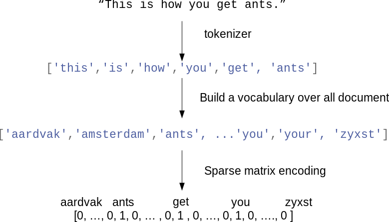
词袋表示
这种表示舍弃了输入文本中的大部分结构,如段落、章节、句子和格式,只计算每个单词在每个文本中的出现频次。
计算词袋有以下步骤:
- 分词(tokenization):将每个文档划分为出现在其中的单词,按空格和标点划分。
- 构建词表(vocabulary building):收集词表,包含出现在任意文档的所有词。
- 编码(encoding):对于每个文档,计算每个单词在文档中的出现频次。(稀疏矩阵存储)
CountVectorizer
- 简单使用
from sklearn.feature_extraction.text import CountVectorizer
vect = CountVectorizer()
vect.fit(bard_words) # train
len(vect.vocabulary_)
vect.vocabulary_
bag_of_words = vect.transform(bard_words) # 词袋表示使用稀疏矩阵存储
bag_of_words.toarray() # 转换成array可视化- 改进单词提取
CountVectorizer使用正则表达式进行分词 "\b\w\w+\b"
指定min_df可以减少特征量,仅使用至少在min_df个文档出现的单词
vect = CountVectorizer(min_df=5).fit(text_train)
X_train = vect.transform(text_train)
feature_names = vect.get_feature_names() # get feature name- 删除停用词
指定stop_words字段
vect = CountVectorizer(min_df=5,stop_words="english").fit(text_train)
X_train = vect.transform(text_train)
TfidfVectorizer
tf-idf方法
tf-idf即词频-逆向文档频率,这种方法对于在某个特定文档经常出现的术语给予很高的权重,对于在语料库中的不同文档经常出现的术语给予较低的权重,因此高权重的术语更有可能概括整个文档的内容.
$$
tfidf(w,d) = tf \log (\frac {N+1}{N_w+1})+1
$$
sklearn
- 结合logisticsRegression进行情感预测
from sklearn.feature_extraction.text import TfidfVectorizer
from sklearn.pipeline import make_pipeline
pipe = make_pipeline(TfidfVectorizer(min_df=5, norm=None),
                     LogisticRegression())
param_grid = {'logisticregression__C': [0.001, 0.01, 0.1, 1, 10]}

grid = GridSearchCV(pipe, param_grid, cv=5)
grid.fit(text_train, y_train)
print("Best cross-validation score: {:.2f}".format(grid.best_score_))- 查看tfidf产生的权重
vectorizer = grid.best_estimator_.named_steps["tfidfvectorizer"]
# transform the training dataset:
X_train = vectorizer.transform(text_train)
# find maximum value for each of the features over dataset:
max_value = X_train.max(axis=0).toarray().ravel()
sorted_by_tfidf = max_value.argsort()
# get feature names
feature_names = np.array(vectorizer.get_feature_names())

print("Features with lowest tfidf:\n{}".format(
      feature_names[sorted_by_tfidf[:20]]))

print("Features with highest tfidf: \n{}".format(
feature_names[sorted_by_tfidf[-20:]]))- 查看回归模型的参数
mglearn.tools.visualize_coefficients(
    grid.best_estimator_.named_steps["logisticregression"].coef_,
    feature_names, n_top_features=40)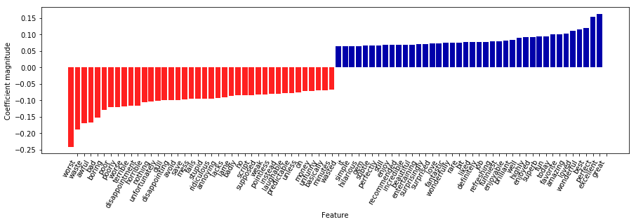
N元分词
n元分词可以保存句子的结构信息.n个词例可以组成一个n-gram.
- 一元分词
cv = CountVectorizer(ngram_range=(1, 1)).fit(bards_words)
print("Vocabulary size: {}".format(len(cv.vocabulary_)))
print("Vocabulary:\n{}".format(cv.get_feature_names()))
- 二元分词
cv = CountVectorizer(ngram_range=(2, 2)).fit(bards_words)
print("Vocabulary size: {}".format(len(cv.vocabulary_)))
print("Vocabulary:\n{}".format(cv.get_feature_names()))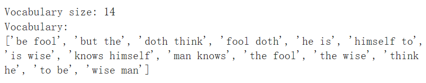
- 三元分词
cv = CountVectorizer(ngram_range=(1, 3)).fit(bards_words)
print("Vocabulary size: {}".format(len(cv.vocabulary_)))
print("Vocabulary:\n{}".format(cv.get_feature_names()))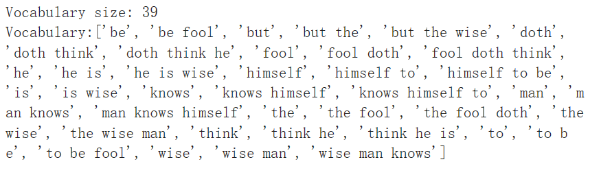
- 热力图表示
# extract scores from grid_search
scores = grid.cv_results_['mean_test_score'].reshape(-1, 3).T
# visualize heat map
heatmap = mglearn.tools.heatmap(
    scores, xlabel="C", ylabel="ngram_range", cmap="viridis", fmt="%.3f",
    xticklabels=param_grid['logisticregression__C'],
    yticklabels=param_grid['tfidfvectorizer__ngram_range'])
plt.colorbar(heatmap)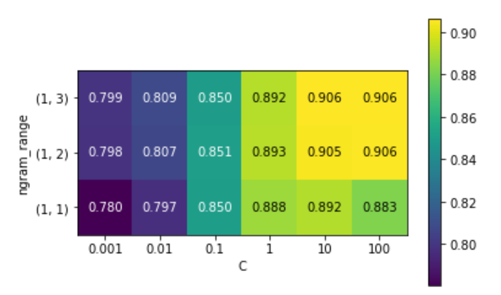
高级分词/词干提取/词形还原
词干提取/词形还原都属于normalization.使用Porter进行词干提取,使用spacy包实现词形还原
import spacy
import nltk

# load spacy's English-language models
en_nlp = spacy.load('en')
# instantiate nltk's Porter stemmer
stemmer = nltk.stem.PorterStemmer()

# define function to compare lemmatization in spacy with stemming in nltk
def compare_normalization(doc):
    # tokenize document in spacy
    doc_spacy = en_nlp(doc)
    # print lemmas found by spacy
    print("Lemmatization:")
    print([token.lemma_ for token in doc_spacy])
    # print tokens found by Porter stemmer
    print("Stemming:")
    print([stemmer.stem(token.norm_.lower()) for token in doc_spacy])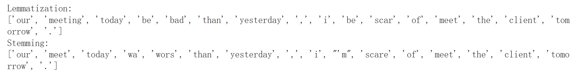
主题建模和文档聚类
使用隐含迪利克雷分布(LDA)进行主题建模.
vect = CountVectorizer(max_features=10000, max_df=.15)
X = vect.fit_transform(text_train)

from sklearn.decomposition import LatentDirichletAllocation
lda = LatentDirichletAllocation(n_topics=10, learning_method="batch",
                                max_iter=25, random_state=0)
# We build the model and transform the data in one step
# Computing transform takes some time,
# and we can save time by doing both at once
document_topics = lda.fit_transform(X)- LDA的components_属性
print("lda.components_.shape: {}".format(lda.components_.shape))
# lda.components_.shape: (10, 10000) 即每个单词对于每个主题的重要性- LDA重要性可视化
# for each topic (a row in the components_), sort the features (ascending).
# Invert rows with [:, ::-1] to make sorting descending
sorting = np.argsort(lda.components_, axis=1)[:, ::-1]
# get the feature names from the vectorizer:
feature_names = np.array(vect.get_feature_names())
# Print out the 10 topics:
mglearn.tools.print_topics(topics=range(10), feature_names=feature_names,
                           sorting=sorting, topics_per_chunk=5, n_words=10)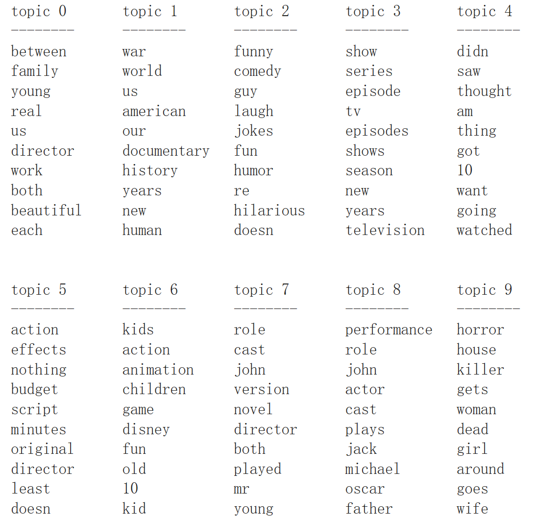
- 查看主题的整体权重
fig, ax = plt.subplots(1, 2, figsize=(10, 10))
topic_names = ["{:>2} ".format(i) + " ".join(words)
               for i, words in enumerate(feature_names[sorting[:, :2]])]
# two column bar chart:
for col in [0, 1]:
    start = col * 50
    end = (col + 1) * 50
    ax[col].barh(np.arange(50), np.sum(document_topics100, axis=0)[start:end])
    ax[col].set_yticks(np.arange(50))
    ax[col].set_yticklabels(topic_names[start:end], ha="left", va="top")
    ax[col].invert_yaxis()
    ax[col].set_xlim(0, 2000)
    yax = ax[col].get_yaxis()
    yax.set_tick_params(pad=130)
plt.tight_layout()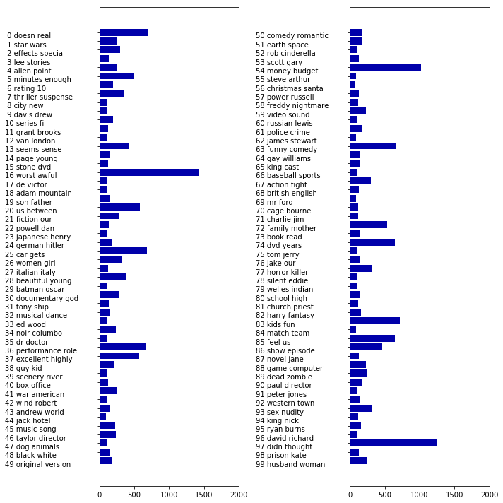
评论