mmcv真的有踩不完的坑，无力吐槽————

简单介绍LoRA，并对LoRA官方源码进行解读，修复了一个bug(可能)

Github: https://github.com/microsoft/LoRA

Arxiv: https://arxiv.org/abs/2106.09685

简单介绍

在LLM微调领域常常听到LoRA及其各种变体，一直以来的印象就是参数量少，不影响推理。今天彻底看看相应的论文和实现。

总结LoRA其实很容易，整篇论文除去实验，只需要一张图和一个公式。

$$ h = W_0x + \Delta Wx = W_0x + B A x \label{eq1} \tag{1} $$

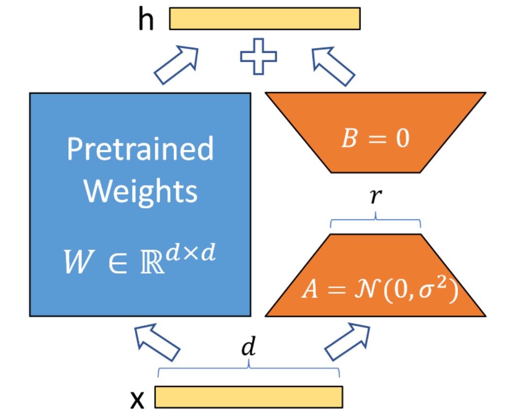
简单来说，LoRA的灵感来自Aghajanyan等人¹，他们发现预训练LLM具有较低的“instrisic dimension”，尽管随机投影到较小的子空间，但仍然可以有效地学习。

也就意味着式$\eqref{eq1}$中的$W$可能是低秩的，那么合理假设：在下游任务的微调过程中，模型权重改变量$\Delta W$也可能是低秩的，那么$\Delta W$就可以使用矩阵$A,B$进行建模。例如$A = matrix(d,r), B = matrix(r, h)$，两者的秩都不会超过$r$,且$r<<min(d,h)$。

这样的好处在于，由于$r$可以非常小(论文里甚至在训GPT-2时取$r=1$)，$A,B$的参数量相较于LLM也很小，微调友好。并且对于不同的下游任务，可以通过切换不同的$\Delta W$来实现task的切换(相当于复用预训练LLM的权重)。部署时，也可以将$\Delta W$合并到$W$中，从而不影响推理性能(与其他微调方法相比，如Adapter)。

源码解读

接下来直接看loralib的官方实现，整体代码还是十分简洁的。库里实现了nn.Embedding/nn.Linear/nn.Conv的LoRA封装。有些实现细节与论文有所出入，以下主要讨论出入部分。

LoRALayer

LoRALayer类的作用主要是定义LoRA中需要用到的一些参数，如rank，scale因子$\alpha$，dropout rate，以及参数是否合并的标志merge_weights等。

class LoRALayer():
    def __init__(
        self, 
        r: int, 
        lora_alpha: int, 
        lora_dropout: float,
        merge_weights: bool,
    ):
        self.r = r
        self.lora_alpha = lora_alpha
        # Optional dropout
        if lora_dropout > 0.:
            self.lora_dropout = nn.Dropout(p=lora_dropout)
        else:
            self.lora_dropout = lambda x: x
        # Mark the weight as unmerged
        self.merged = False
        self.merge_weights = merge_weights

Linear

先从Linear层说起，init函数中，定义了$A,B$两个矩阵。

这里A矩阵(B矩阵同理)定义成(r, in_features)的shape，而不是(in_features, r) , 应该是为了和nn.Linear.weight.data的shape: (out_features, in_features)保持一致

# Actual trainable parameters
if r > 0:
    self.lora_A = nn.Parameter(self.weight.new_zeros((r, in_features)))
    self.lora_B = nn.Parameter(self.weight.new_zeros((out_features, r)))

值得注意的是这里A矩阵使用的是kaiming_uniform_。

nn.init.kaiming_uniform_(self.lora_A, a=math.sqrt(5))
nn.init.zeros_(self.lora_B)

训练时，如果是train mode，会将$\Delta W$与$W$分离；如果是eval mode，则会将其合并，提高推理速度。这里的$\Delta W$就是$B @ A$。

def train(self, mode: bool = True):
    def T(w):
        return w.transpose(0, 1) if self.fan_in_fan_out else w
    nn.Linear.train(self, mode)
    if mode:
        if self.merge_weights and self.merged:
            # Make sure that the weights are not merged
            if self.r > 0:
                self.weight.data -= T(self.lora_B @ self.lora_A) * self.scaling
            self.merged = False
    else:
        if self.merge_weights and not self.merged:
            # Merge the weights and mark it
            if self.r > 0:
                self.weight.data += T(self.lora_B @ self.lora_A) * self.scaling
            self.merged = True      

forward函数如下, 如果权重没有merge，分别计算结果相加即可。

def forward(self, x: torch.Tensor):
    def T(w):
        return w.transpose(0, 1) if self.fan_in_fan_out else w
    if self.r > 0 and not self.merged:
        result = F.linear(x, T(self.weight), bias=self.bias)            
        result += (self.lora_dropout(x) @ self.lora_A.transpose(0, 1) @ self.lora_B.transpose(0, 1)) * self.scaling
        return result
    else:
        return F.linear(x, T(self.weight), bias=self.bias)

Embedding

Embedding层与其他层不太一样，A矩阵的作用是为num_embeddings个值分配对应的向量，维度为r，B的作用是进一步将向量映射到embedding_dim维度。

这里A更合适的shape应该是(num_embeddings, r)，否则后续会出现很多transpose操作

这里这么写应该是和其他layer保持一致

self.lora_A = nn.Parameter(self.weight.new_zeros((r, num_embeddings)))
self.lora_B = nn.Parameter(self.weight.new_zeros((embedding_dim, r)))

因此初始化与论文的图不太一样，这里是将A矩阵置0。

nn.init.zeros_(self.lora_A)
nn.init.normal_(self.lora_B)

forward函数也是先通过A矩阵embedding到维度r，再和B矩阵相乘得到最后结果。

if self.r > 0 and not self.merged:
    result = nn.Embedding.forward(self, x)
    after_A = F.embedding(
        x, self.lora_A.transpose(0, 1), self.padding_idx, self.max_norm,
        self.norm_type, self.scale_grad_by_freq, self.sparse
    )
    result += (after_A @ self.lora_B.transpose(0, 1)) * self.scaling
    return result
else:
    return nn.Embedding.forward(self, x)

MergedLinear

这个类的作用主要是和Transformer的QKV结构适配，官方示例如下。

# ===== Before =====
# qkv_proj = nn.Linear(d_model, 3*d_model)
# ===== After =====
# Break it up (remember to modify the pretrained checkpoint accordingly)
q_proj = lora.Linear(d_model, d_model, r=8)
k_proj = nn.Linear(d_model, d_model)
v_proj = lora.Linear(d_model, d_model, r=8)
# Alternatively, use lora.MergedLinear (recommended)
qkv_proj = lora.MergedLinear(d_model, 3*d_model, r=8, enable_lora=[True, False, True])

大部分代码对于QKV的映射都是使用一个nn.Linear(d_model, 3*d_model)解决，但是LoRA有时候只想应用到QV上，这时候可以把Linear分成三个Linear，也可以使用MergedLinear。

MergedLinear实现其实有点像Bert里的Attention head pruning。lora_ind判断当前哪些输出需要用到LoRA，A矩阵是sum(enable_lora)个(r, in_features)矩阵，B矩阵是(out_features // len(enable_lora) * sum(enable_lora), r)的矩阵，这里对out_features进行了剪枝。

B矩阵其实也指后续AB合并用到的Conv1d.weight，shape为(final_out_features, in_channels/groups, kernel_size)

if r > 0 and any(enable_lora):
    self.lora_A = nn.Parameter(
    self.weight.new_zeros((r * sum(enable_lora), in_features)))
    self.lora_B = nn.Parameter(
    self.weight.new_zeros((out_features // len(enable_lora) * sum(enable_lora), r))
    ) # weights for Conv1D with groups=sum(enable_lora)
    self.scaling = self.lora_alpha / self.r
    # Freezing the pre-trained weight matrix
    self.weight.requires_grad = False
    # Compute the indices
    self.lora_ind = self.weight.new_zeros(
    (out_features, ), dtype=torch.bool
    ).view(len(enable_lora), -1)
    self.lora_ind[enable_lora, :] = True
    self.lora_ind = self.lora_ind.view(-1)

这里A、B矩阵的合并用到了1d卷积操作，具体shape可以见注释。groups的作用是对于不同输入(QKV)分别卷积。

def zero_pad(self, x):
    result = x.new_zeros((len(self.lora_ind), *x.shape[1:]))
    result[self.lora_ind] = x
    return result

def merge_AB(self):
    def T(w):
        return w.transpose(0, 1) if self.fan_in_fan_out else w
    delta_w = F.conv1d(
        self.lora_A.unsqueeze(0), # shape: [1, r * sum(enable_lora), in_features]
        self.lora_B.unsqueeze(-1), # shape: [out_features // len(enable_lora) * sum(enable_lora), r, 1]
        groups=sum(self.enable_lora)
    ).squeeze(0) # shape: [out_features // len(enable_lora) * sum(enable_lora), in_features]
    return T(self.zero_pad(delta_w)) # after zero_pad, shape: [out_features, in_features]

经过实测，这里的合并操作也可以写成以下形式，可能更方便理解

delta_w = (self.lora_B.view(sum(enable_lora), out_features//len(enable_lora), r) @ self.lora_A.view(sum(enable_lora), r, in_features)).view(-1,in_features)      

ConvLoRA

ConvLoRA提供了1d/2d/3d卷积的封装，主要看AB矩阵的定义。这里的self.conv.groups与之前提到的一致，系卷积中的分组。

if r > 0:
    self.lora_A = nn.Parameter(
    self.conv.weight.new_zeros((r * kernel_size, in_channels * kernel_size))
)
    self.lora_B = nn.Parameter(
    self.conv.weight.new_zeros((out_channels//self.conv.groups*kernel_size, r*kernel_size))
)

AB矩阵的合并也很简单，直接(self.lora_B @ self.lora_A).view(self.conv.weight.shape)即可。

当然这里的问题在于(self.lora_B @ self.lora_A)的shape只能reshape到(out_channels, in_channels//self.conv.groups, kernel_size, kernel_size即2d卷积weight的shape。所以这种写法是否可以支持1d/3d，暂时打一个问号。

并且这里AB矩阵的rank最大可以是r * kernel_size，为什么不把kernel_size写到另外一边？

比如写成如下形式，正好也解决了Conv1d/3d的问题~

2023.12.20 Updates: Github上原来已经有这个问题的讨论了😀 https://github.com/microsoft/LoRA/issues/115

# Conv2d
self.lora_A = nn.Parameter(
    self.conv.weight.new_zeros((r, in_channels * kernel_size * kernel_size))
)
    self.lora_B = nn.Parameter(
    self.conv.weight.new_zeros((out_channels//self.conv.groups*kernel_size, r))
# Conv3d
self.lora_A = nn.Parameter(
    self.conv.weight.new_zeros((r, in_channels * kernel_size * kernel_size * kernel_size))
)
self.lora_B = nn.Parameter(
    self.conv.weight.new_zeros((out_channels//self.conv.groups*kernel_size, r))
# Conv1d
self.lora_A = nn.Parameter(
    self.conv.weight.new_zeros((r, in_channels * kernel_size))
)
self.lora_B = nn.Parameter(
    self.conv.weight.new_zeros((out_channels//self.conv.groups*kernel_size, r))

DDPM中建模的$q(\mathbf{x}_{t-1} \vert \mathbf{x}_t, \mathbf{x}_0)$满足正态分布，

$$ q(\mathbf{x}_{t-1} \vert \mathbf{x}_t, \mathbf{x}_0) = \mathcal{N}(\mathbf{x}_{t-1}; \tilde{\boldsymbol{\mu}}(\mathbf{x}_t, \mathbf{x}_0), \tilde{\beta}_t \mathbf{I}) \\ \tilde{\beta}_t = \frac{1 - \bar{\alpha}_{t-1}}{1 - \bar{\alpha}_t} \cdot \beta_t $$

DDIM中建模的$q_\sigma(\mathbf{x}_{t-1} \vert \mathbf{x}_t, \mathbf{x}_0)$如下，第一个等式二三步用到了重参数技巧和多个独立高斯分布的等价形式，

$$ \begin{aligned} \mathbf{x}_{t-1} &= \sqrt{\bar{\alpha}_{t-1}}\mathbf{x}_0 + \sqrt{1 - \bar{\alpha}_{t-1}}\boldsymbol{\epsilon}_{t-1} \\ &= \sqrt{\bar{\alpha}_{t-1}}\mathbf{x}_0 + \sqrt{1 - \bar{\alpha}_{t-1} - \sigma_t^2} \boldsymbol{\epsilon}_t + \sigma_t\boldsymbol{\epsilon} \\ &= \sqrt{\bar{\alpha}_{t-1}}\mathbf{x}_0 + \sqrt{1 - \bar{\alpha}_{t-1} - \sigma_t^2} \frac{\mathbf{x}_t - \sqrt{\bar{\alpha}_t}\mathbf{x}_0}{\sqrt{1 - \bar{\alpha}_t}} + \sigma_t\boldsymbol{\epsilon} \\ q_\sigma(\mathbf{x}_{t-1} \vert \mathbf{x}_t, \mathbf{x}_0) &= \mathcal{N}(\mathbf{x}_{t-1}; \sqrt{\bar{\alpha}_{t-1}}\mathbf{x}_0 + \sqrt{1 - \bar{\alpha}_{t-1} - \sigma_t^2} \frac{\mathbf{x}_t - \sqrt{\bar{\alpha}_t}\mathbf{x}_0}{\sqrt{1 - \bar{\alpha}_t}}, \sigma_t^2 \mathbf{I}) \end{aligned} $$

DDIM中的的$\sigma_t$与DDPM中的$\tilde{\beta_t}$保持一致，并且添加了一个可学习参数控制方差，

$$ \sigma^2_t = \eta \cdot \tilde{\beta}_t $$

当$\eta=0$时，采样过程是确定的；当$\eta=1$时，退化成DDPM的形式，以下给出推导，

$$ \begin{aligned} \mu_{\mathbf{x}_{t-1}} &= \sqrt{\bar{\alpha}_{t-1}}\mathbf{x}_0 + \sqrt{1 - \bar{\alpha}_{t-1} - \sigma_t^2} \frac{\mathbf{x}_t - \sqrt{\bar{\alpha}_t}\mathbf{x}_0}{\sqrt{1 - \bar{\alpha}_t}} \\ &= \sqrt{\bar{\alpha}_{t-1}}\mathbf{x}_0 + \sqrt{1 - \bar{\alpha}_{t-1} - \tilde{\beta}_t} \frac{\mathbf{x}_t - \sqrt{\bar{\alpha}_t}\mathbf{x}_0}{\sqrt{1 - \bar{\alpha}_t}} \\ &= \sqrt{\bar{\alpha}_{t-1}}\mathbf{x}_0 + \sqrt{1 - \bar{\alpha}_{t-1} - \frac{(1 - \bar{\alpha}_{t-1}) \cdot (1 - \alpha_t)}{1 - \bar{\alpha}_t}} \frac{\mathbf{x}_t - \sqrt{\bar{\alpha}_t}\mathbf{x}_0}{\sqrt{1 - \bar{\alpha}_t}} \\ &= (\sqrt{\bar{\alpha}_{t-1}} + \sqrt{1 - \bar{\alpha}_{t-1} - \frac{(1 - \bar{\alpha}_{t-1}) \cdot (1 - \alpha_t)}{1 - \bar{\alpha}_t}} \cdot \frac{ - \sqrt{\bar{\alpha}_t}}{\sqrt{1 - \bar{\alpha}_t}}) \cdot \mathbf{x}_0 + \sqrt{1 - \bar{\alpha}_{t-1} - \frac{(1 - \bar{\alpha}_{t-1}) \cdot (1 - \alpha_t)}{1 - \bar{\alpha}_t}} \cdot \frac{\mathbf{x}_t}{\sqrt{1 - \bar{\alpha}_t}} \\ &= (\sqrt{\bar{\alpha}_{t-1}} + \sqrt{(1 - \bar{\alpha}_{t-1}) \cdot (1 - \frac{1 - \alpha_t}{1 - \bar{\alpha}_t})} \cdot \frac{ - \sqrt{\bar{\alpha}_t}}{\sqrt{1 - \bar{\alpha}_t}}) \cdot \mathbf{x}_0 + \sqrt{(1 - \bar{\alpha}_{t-1}) \cdot (1 - \frac{1 - \alpha_t}{1 - \bar{\alpha}_t})} \cdot \frac{\mathbf{x}_t}{\sqrt{1 - \bar{\alpha}_t}} \\ &= (\sqrt{\bar{\alpha}_{t-1}} + \sqrt{(1 - \bar{\alpha}_{t-1}) \cdot \frac{\alpha_t - \bar\alpha_t}{1 - \bar{\alpha}_t}} \cdot \frac{ - \sqrt{\bar{\alpha}_t}}{\sqrt{1 - \bar{\alpha}_t}}) \cdot \mathbf{x}_0 + \sqrt{(1 - \bar{\alpha}_{t-1}) \frac{\alpha_t - \bar\alpha_t}{1 - \bar{\alpha}_t}} \cdot \frac{\mathbf{x}_t}{\sqrt{1 - \bar{\alpha}_t}} \\ &= (\sqrt{\bar{\alpha}_{t-1}} + \sqrt{1 - \bar{\alpha}_{t-1}} \cdot \frac{\sqrt{\alpha_t - \bar\alpha_t}}{\sqrt{{1 - \bar{\alpha}_t}}} \cdot \frac{ - \sqrt{\bar{\alpha}_t}}{\sqrt{1 - \bar{\alpha}_t}}) \cdot \mathbf{x}_0 + \sqrt{1 - \bar{\alpha}_{t-1}} \cdot \frac{\sqrt{\alpha_t - \bar\alpha_t}}{\sqrt{{1 - \bar{\alpha}_t}}} \cdot \frac{\mathbf{x}_t}{\sqrt{1 - \bar{\alpha}_t}} \\ &= (\sqrt{\bar{\alpha}_{t-1}} - \sqrt{1 - \bar{\alpha}_{t-1}} \cdot \frac{\sqrt{1 - \bar\alpha_{t-1}} \cdot \sqrt{\alpha_t}}{\sqrt{{1 - \bar{\alpha}_t}}} \cdot \frac{\sqrt{\bar{\alpha}_t}}{\sqrt{1 - \bar{\alpha}_t}}) \cdot \mathbf{x}_0 + \sqrt{1 - \bar{\alpha}_{t-1}} \cdot \frac{\sqrt{1 - \bar\alpha_{t-1}} \cdot \sqrt{\alpha_t}}{\sqrt{{1 - \bar{\alpha}_t}}} \cdot \frac{\mathbf{x}_t}{\sqrt{1 - \bar{\alpha}_t}} \\ &= (\sqrt{\bar{\alpha}_{t-1}} - \frac{\sqrt{\alpha_t} \cdot \sqrt{\bar\alpha_t} \cdot (1 - \bar\alpha_{t-1})}{1 - \bar\alpha_{t}}) \cdot \mathbf{x}_0 + \frac{\sqrt{\alpha_t} \cdot (1 - \bar\alpha_{t-1}) \cdot \mathbf{x}_t}{1 - \bar\alpha_{t}} \\ &= (\frac{\sqrt{\bar{\alpha}_{t-1}} - \bar\alpha_t \cdot \sqrt{\bar{\alpha}_{t-1}} - \sqrt{\alpha_t} \cdot \sqrt{\bar\alpha_t} \cdot + \sqrt{\alpha_t} \cdot \sqrt{\bar\alpha_t} \cdot \bar\alpha_{t-1}}{1 - \bar\alpha_{t}}) \cdot \mathbf{x}_0 + \frac{\sqrt{\alpha_t} \cdot (1 - \bar\alpha_{t-1}) \cdot \mathbf{x}_t}{1 - \bar\alpha_{t}} \\ &= (\frac{\sqrt{\bar{\alpha}_{t-1}} - \bar\alpha_t \cdot \sqrt{\bar{\alpha}_{t-1}} - \sqrt{\alpha_{t-1}} \cdot \bar\alpha_t + \sqrt{\bar\alpha_{t-1}} \cdot \bar\alpha_t}{1 - \bar\alpha_{t}}) \cdot \mathbf{x}_0 + \frac{\sqrt{\alpha_t} \cdot (1 - \bar\alpha_{t-1}) \cdot \mathbf{x}_t}{1 - \bar\alpha_{t}} \\ &= (\frac{\sqrt{\bar{\alpha}_{t-1}} - \sqrt{\alpha_{t-1}} \cdot \bar\alpha_t }{1 - \bar\alpha_{t}}) \cdot \mathbf{x}_0 + \frac{\sqrt{\alpha_t} \cdot (1 - \bar\alpha_{t-1}) \cdot \mathbf{x}_t}{1 - \bar\alpha_{t}} \\ &= \mu_{\mathbf{x}_{t-1}}^{DDPM} \end{aligned} $$

最近看到一个写的挺好的多任务框架(https://github.com/SwinTransformer/AiT，参考了detectron2)，分享一下~

多任务训练一般分为两种：data mixing 和 batch mixing。简单来说，对于前者，一个batch中的样本可以来自不同任务，而后者一个batch中任务都是一样的。两者相比，后者实现更加容易，效率更高，并且做数据增强也更方便一点(由Pix2Seq提出，但其实数据增强我认为并不是两者的主要差异)。

先给出我写的一个batch mixing的例子(来自JJJYmmm/Pix2SeqV2-Pytorch)：

def get_multi_task_loaders(tokenizer,tasks):

    assert set(tasks) <= set(['detection', 'keypoint', 'segmentation', 'captioning'])

    train_loaders = {}
    valid_loaders = {}

    if 'detection' in tasks:
        detection_train_loader, detection_valid_loader = detection_loaders(
        CFG.dir_root, tokenizer, CFG.img_size, CFG.batch_size, CFG.max_len, tokenizer.PAD_code)
        train_loaders['detection'] = detection_train_loader
        valid_loaders['detection'] = detection_valid_loader
   
    if 'keypoint' in tasks: 
        keypoint_train_loader, keypoint_valid_loader = keypoint_loaders(
        CFG.dir_root, tokenizer,person_kps_info, CFG.img_size, CFG.batch_size, CFG.max_len, tokenizer.PAD_code)
        train_loaders['keypoint'] = keypoint_train_loader
        valid_loaders['keypoint'] = keypoint_valid_loader

    if 'segmentation' in tasks: 
        segmentation_train_loader, segmentation_valid_loader = segmentation_loaders(
        CFG.dir_root, tokenizer,person_kps_info, CFG.img_size, CFG.batch_size, CFG.max_len, tokenizer.PAD_code)
        train_loaders['segmentation'] = segmentation_train_loader
        valid_loaders['segmentation'] = segmentation_valid_loader

    if 'captioning' in tasks:
        img_caption_train_loader, img_caption_valid_loader = img_caption_loaders(
        CFG.dir_root, tokenizer,vocab, CFG.img_size, CFG.batch_size, CFG.max_len, tokenizer.PAD_code)
        train_loaders['captioning'] = img_caption_train_loader
        valid_loaders['captioning'] = img_caption_valid_loader
    
    return train_loaders, valid_loaders

以上代码首先维护一个多任务的dataloader字典，在这里之前(即创建dataset)就可以针对不同任务做对应的数据增强。

# get longest dataloader
epoch_size = 0
longest_loader = None
for name, loader in train_loaders.items():
    if len(loader) > epoch_size:
        epoch_size = len(loader)
        longest_loader = name

# create iter for dataloaders
loader_iters = dict()
for k, v in train_loaders.items():
    if k != longest_loader:
        loader_iters[k] = iter(v)

# iter longest dataloader
tqdm_object = tqdm(train_loaders[longest_loader], total=len(train_loaders[longest_loader]))
for iteration,(x, y, init_lens) in enumerate(tqdm_object):

    optimizer.zero_grad()
        
    total_loss = torch.zeros(1, requires_grad=False, device=CFG.device)
    total_batch = x.size(0)
    # loss_1
    loss = cal_loss_multi_task(model, criterion, x, y, init_lens, task_id = task_ids[longest_loader])
    total_loss = total_loss + loss.item() * task_weights[longest_loader]
    loss *= task_weights[longest_loader] # mul weight
    loss.backward()
    # calculate other tasks' loss
    for k, v in loader_iters.items():
        try:
            (x, y, init_lens) = next(v)
        except StopIteration: # recover other tasks' iter
            loader_iters[k] = iter(train_loaders[k])
            (x, y, init_lens) = next(loader_iters[k])
        total_batch += x.size(0)
        # loss_i
        loss = cal_loss_multi_task(model, criterion, x, y, init_lens, task_id=task_ids[k])
        total_loss = total_loss + loss.item() * task_weights[k]
        loss *= task_weights[k]
        loss.backward()

    # total_loss.backward()
    optimizer.step()

训练时，首先确定batch数最多的任务(数据集A)，把它作为训练的最外层，这一部分和单任务训练一致，对于其他任务，则分别创建一个迭代器iterator负责取数据。之后在循环数据集A的时候，每次算出loss_A后，会从其他迭代器中取出对应的数据并计算loss_B/loss_C...，之后根据任务权重对loss进行加权平均，并进行反向传播。

在上述代码中，为了节省显存，每次计算完loss，我都直接乘上权重反向传播了，这个好处在于，每个loss计算完后对应的计算图会被自动释放，如果显式显出加权平均，那么所有任务的计算图都会被保留~

可以看出，batch mixing其实只是在训练过程中加入多个数据集的batch，然后分别算出loss并反向传播罢了。(data mixing也差不多，只是粒度更细一点)

关于data mixing，其实就比batch mixing多了一步操作，就是把所有的数据集拼起来，然后对于每个样本都添加一个字段表示任务。取数据的时候直接从大数据集里面取就可以了。

class ConcatDataset(Dataset[T_co]):
    r"""Dataset as a concatenation of multiple datasets.

    This class is useful to assemble different existing datasets.

    Args:
        datasets (sequence): List of datasets to be concatenated
    """
    datasets: List[Dataset[T_co]]
    cumulative_sizes: List[int]

    @staticmethod
    def cumsum(sequence):
        r, s = [], 0
        for e in sequence:
            l = len(e)
            r.append(l + s)
            s += l
        return r

    def __init__(self, datasets: Iterable[Dataset]) -> None:
        super(ConcatDataset, self).__init__()
        self.datasets = list(datasets)
        assert len(self.datasets) > 0, 'datasets should not be an empty iterable'  # type: ignore[arg-type]
        for d in self.datasets:
            assert not isinstance(d, IterableDataset), "ConcatDataset does not support IterableDataset"
        self.cumulative_sizes = self.cumsum(self.datasets)

    def __len__(self):
        return self.cumulative_sizes[-1]

    def __getitem__(self, idx):
        if idx < 0:
            if -idx > len(self):
                raise ValueError("absolute value of index should not exceed dataset length")
            idx = len(self) + idx
        dataset_idx = bisect.bisect_right(self.cumulative_sizes, idx)
        if dataset_idx == 0:
            sample_idx = idx
        else:
            sample_idx = idx - self.cumulative_sizes[dataset_idx - 1]
        return self.datasets[dataset_idx][sample_idx]

    @property
    def cummulative_sizes(self):
        warnings.warn("cummulative_sizes attribute is renamed to "
                      "cumulative_sizes", DeprecationWarning, stacklevel=2)
        return self.cumulative_sizes

到这里也就知道，data mixing的数据增强也很方便，在拼接数据集之前，各个数据集定义自己的增强方式即可。但是data mixing的最大问题在于：训练过程中，需要循环batch里的每个样本，根据任务的不同分配给不同的Heads处理loss，并行度其实很差。当然，对于大模型训练来说，有时候单张GPU就放一个样本，那这个劣势就相当于没有了~

最后总结就是，data mixing相比于batch mixing，任务粒度更细，并且对于多任务的支持更好(不像batch mixing每加一个任务就要改train代码，data mixing只需要写好数据集和对应处理的Head即可)，但是并行度相比于batch mixing较差。

复现多卡训练项目经常会遇到一些匪夷所思的问题，包括但不限于numpy<1.2.0 && numpy>=1.2.0，OSError: [Errno 12] 。以下给出尽可能"少犯错"的几个步骤：

• 拿到一个项目，首先检查包依赖(如requirements.txt)，如果使用conda管理虚拟环境，建议每个项目都创建一个env，conda一般会存有各个包的cache，所以不用担心重新搭建一个环境的时间成本；如果作者提供了docker，优先使用docker
• 有些包会存在历史依赖，最经典的是numpy.float/numpy.int在numpy>=1.2.0后弃用，而有些包如boundary-iou还是沿用了旧版本的写法，所以遇到这种情况直接对着报错改包就行(如np.float->np.float64)，当然也可以尝试版本回退
• 对于深度学习项目，如果允许先拿一张卡跑，因为多卡多进程debug信息很难处理
• 对于dataloader，统一先设置num_workers=0，有时候线程过多也会导致错误(例如共享内存shm不足导致的bus error)，另外windows下跑项目我记得这个值必须为0
• batch_size_per_GPU=1有时候很有用，特别是对网络大小没什么概念的时候(当然这个也是最好debug的了，谁会不懂OOM呢[哭])

• 多卡训练debug比较麻烦，网上有很多Vscode/Pycharm方案，这里给一个最原始的pdb注入方式，一般可以处理除了IPC以外的大部分错误了,在想要打断点的地方插入这两行代码即可，调试方式跟gdb差不多

  import pdb
  pdb.set_trace()

剩下的以后想到再补充~